
How to Grey Out Cells Based on Another Column or Dropdown List Choice in Excel

Making certain cells in Excel visually distinct by graying them out based on another column’s value or a dropdown list selection can significantly enhance your data management. This technique is not just about aesthetics; it’s a practical way to highlight or de-emphasize data dynamically, making your spreadsheets more intuitive and user-friendly. Whether you’re a beginner or a seasoned Excel user, follow these simple steps to master this useful skill.
Step 1: Prepare Your Spreadsheet
Start by entering your data into the spreadsheet or setting up your dropdown list. This foundational step ensures that you have the content ready for conditional formatting.

Step 2: Access Conditional Formatting
Highlight the cells you wish to conditionally format (grey out) based on another column’s value or a dropdown list choice. Navigate to the Home tab, find the Styles group, and click on Conditional Formatting. This powerful tool allows you to apply specific formats to cells that meet certain criteria, making it easier to visualize and interpret your data.

Step 3: Initiate a New Rule
In the Conditional Formatting menu, select New Rule to open the rule configuration dialog box. This is where you’ll define the condition that triggers the graying out of cells.
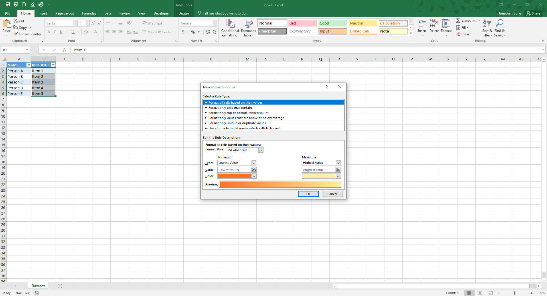
Step 4: Specify Your Condition
Within the dialog box, choose Format only cells that contain. Then, under the section labeled Format only cells with, select either equal to or not equal to, depending on what your condition requires. In the adjacent box, enter the value or cell reference that, when matched, will trigger the formatting. This step is crucial as it determines which cells will be highlighted based on your specified condition.

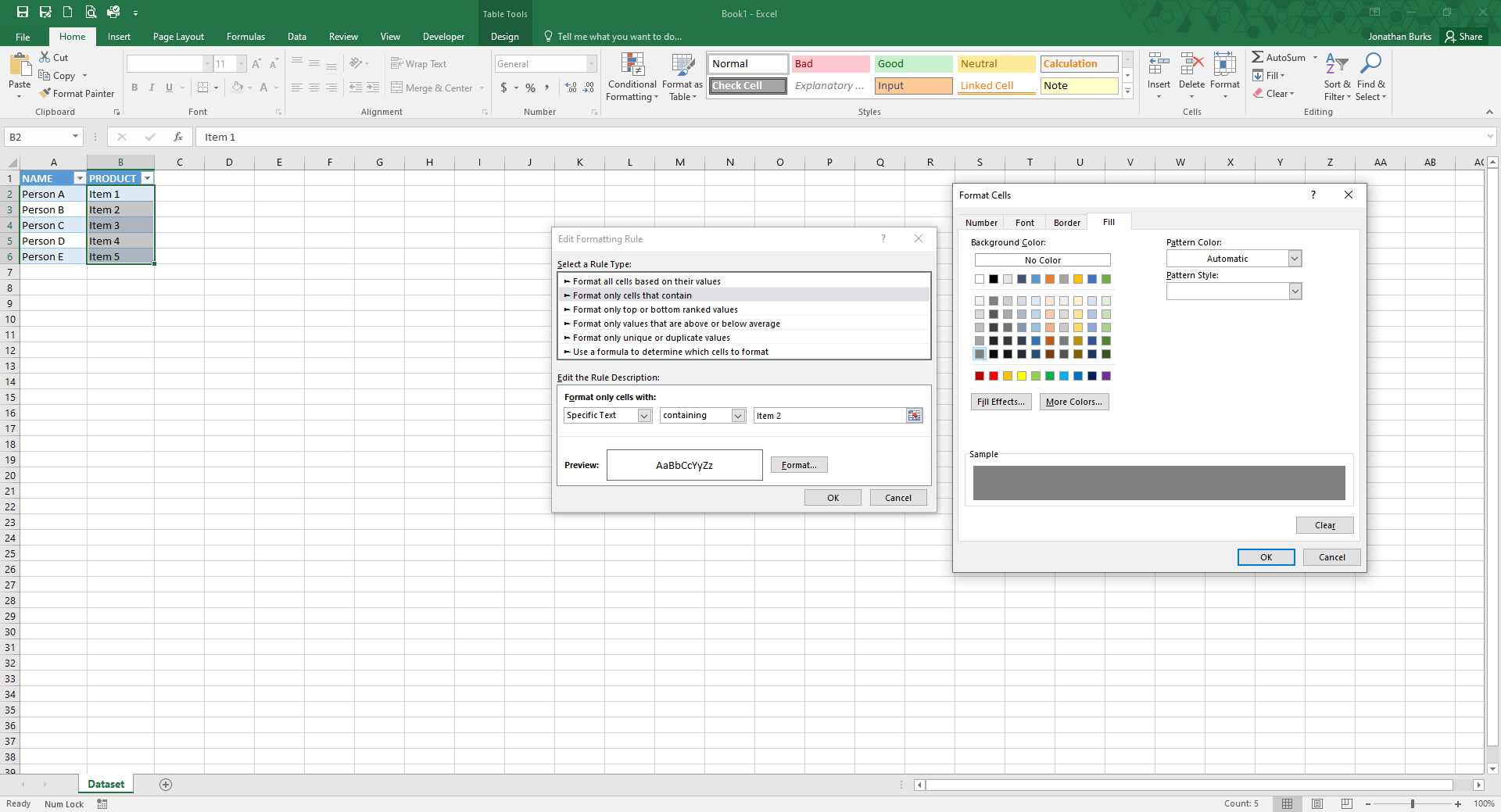
Step 5: Choose Your Formatting
Click the Format button to select how the cells will look when they meet the condition. Go to the Fill tab, select a shade of grey that suits your preference, and press OK. This visual distinction will make it easy to spot which data points are currently relevant or need attention.
Step 6: Apply and Review
Finalize by clicking OK to apply the conditional formatting rule. Review your spreadsheet to see the cells grey out dynamically, based on the condition you’ve set. This immediate visual feedback confirms that your rule is working as intended.
By following these steps, you’ll not only make your spreadsheets more visually organized but also enhance the way you interact with your data. Conditional formatting, especially graying out cells based on specific criteria, is a simple yet powerful technique to elevate your Excel skills and make your data work for you.