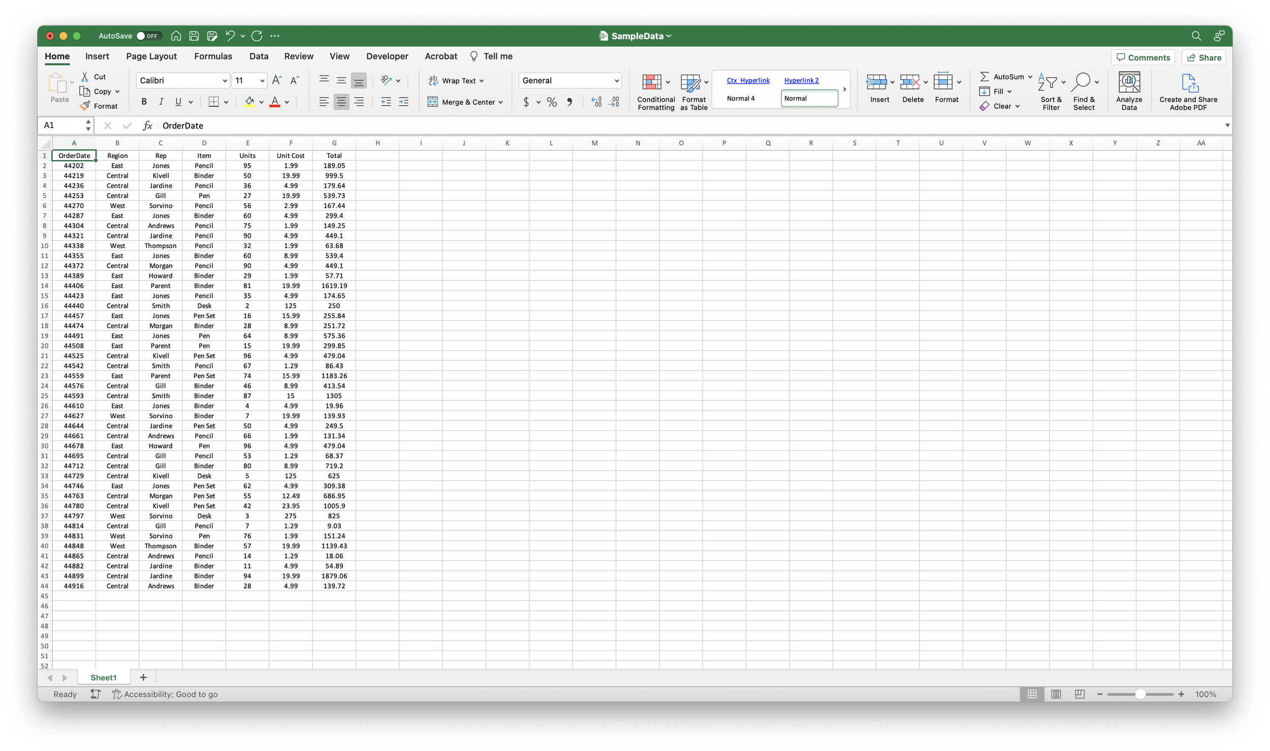
How to Use Conditional Summing Functions in Excel

Conditional summing functions in Microsoft Excel allow you to calculate sums based on specific conditions or criteria. These functions are helpful when you want to sum only the values that meet certain requirements within a dataset. In this tutorial, we'll guide you through the steps to use conditional summing functions in Excel.

Step 1: Open Your Excel Worksheet

1. Open the Excel workbook containing the data you want to perform conditional summing on.

Step 2: SUMIF Function - Summing Values Based on a Single Condition

1. Identify the range of cells that you want to sum based on a condition.
2. Decide on the condition that must be met for the cells to be included in the sum.

Step 3: Use the SUMIF Function

1. Select the cell where you want the sum to appear.
2. Enter the SUMIF function in the formula bar. The basic syntax of the SUMIF function is as follows:

   =SUMIF(range, criteria, [sum_range])

   • range: The range of cells that will be evaluated based on the condition.
   • criteria: The condition that cells must meet to be included in the sum. This can be a specific value, expression, or text.
   • sum_range (optional): The range of cells whose corresponding values will be summed. If omitted, the function will use the range as the sum_range.

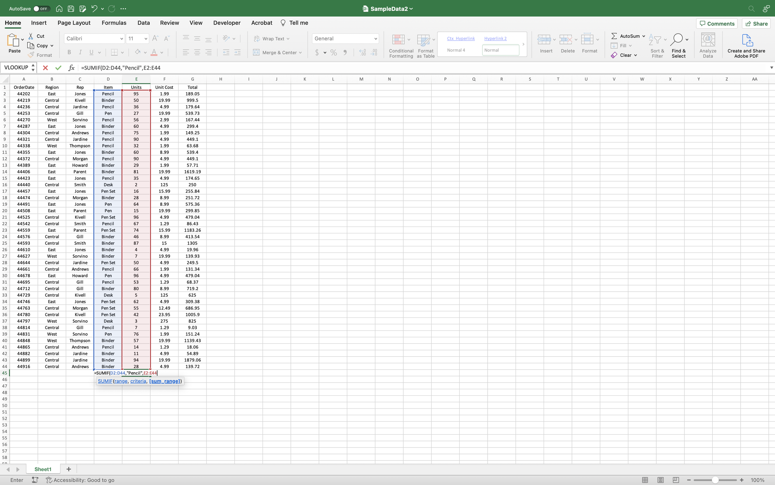
Step 4: Example of Using the SUMIF Function

1. For example, if you have a list of sales and want to find the total sales for a specific product (e.g., "Widget X"), you would use the following formula:

   =SUMIF(A2:A10, "Widget X", B2:B10)

Here, "A2:A10" is the range containing product names, "Widget X" is the condition, and "B2:B10" is the range containing sales values.

Step 5: SUMIFS Function - Summing Values Based on Multiple Conditions

1. If you have multiple conditions, you can use the SUMIFS function.
2. Identify the ranges of cells that you want to evaluate based on different criteria.

Step 6: Use the SUMIFS Function

1. Select the cell where you want the sum to appear.

2. Enter the SUMIFS function in the formula bar. The basic syntax of the SUMIFS function is as follows:

   =SUMIFS(sum_range, criteria_range1, criteria1, [criteria_range2, criteria2], ...)

   • sum_range: The range of cells whose corresponding values will be summed.
   • criteria_range1: The first range of cells that will be evaluated based on the first condition.
   • criteria1: The first condition that cells in criteria_range1 must meet to be included in the sum.
   • [criteria_range2, criteria2]: Additional pairs of criteria ranges and conditions can be added as needed.

Step 7: Example of Using the SUMIFS Function

1. For example, if you have a list of sales with multiple criteria, such as finding the total sales for "Widget X" in a specific region (e.g., "East"), you would use the following formula:

   =SUMIFS(C2:C10, A2:A10, "Widget X", B2:B10, "East")

Here, "C2:C10" is the range containing sales values, "A2:A10" is the range containing product names, "Widget X" is the condition for products, "B2:B10" is the range containing region names, and "East" is the condition for the region.

Step 8: SUMPRODUCT Function - Summing Values with Multiple Criteria (More Complex Scenarios)

1. For even more complex scenarios, you can use the SUMPRODUCT function with arrays to sum values based on multiple conditions.

Step 9: Example of Using the SUMPRODUCT Function

1. For example, if you have sales data with multiple criteria such as product, region, and month, and you want to sum sales for "Widget X" in "East" region for the month of "January," you would use the following formula:

   =SUMPRODUCT((A2:A10="Widget X")(B2:B10="East")(D2:D10="January"), C2:C10)

Here, "A2:A10" is the range containing product names, "B2:B10" is the range containing region names, "D2:D10" is the range containing month names, and "C2:C10" is the range containing sales values.

Step 10: Saving the Workbook

1. Save your Excel workbook to retain the conditional summing formulas and data for future use.

Step 11: Closing Excel

1. When you're done working on your spreadsheet, go to the "File" menu and select "Close" to exit Excel.

Congratulations! You've successfully learned how to use conditional summing functions in Microsoft Excel. With these functions, you can efficiently calculate sums based on specific conditions, allowing you to analyze and aggregate data effectively in your worksheets.