How to Use the MATCH() Function in Excel

The MATCH() function in Excel is a powerful tool that allows you to find the relative position of a specific item within a range or array. It is commonly used in combination with other functions to perform advanced lookups and data analysis. In this article, we will guide you through the process of using the MATCH() function in Excel.

Syntax of MATCH() Function:

Before we delve into its usage, let's understand the syntax of the MATCH() function:

=MATCH(lookup_value, lookup_array, [match_type])

• lookup_value: The value you want to find within the lookup_array.
• lookup_array: The range or array where you want to search for the lookup_value.
• [match_type]: An optional parameter that specifies the type of match. The available options are:
  • 1 (or omitted): Finds the largest value that is less than or equal to the lookup_value (sorted in ascending order).
  • 0: Finds an exact match for the lookup_value (lookup_array must be sorted in ascending order).
  • -1: Finds the smallest value that is greater than or equal to the lookup_value (sorted in descending order).

Step-by-Step Guide to Using the MATCH() Function:

Let's walk through an example of how to use the MATCH() function to find the relative position of a specific value within a range:

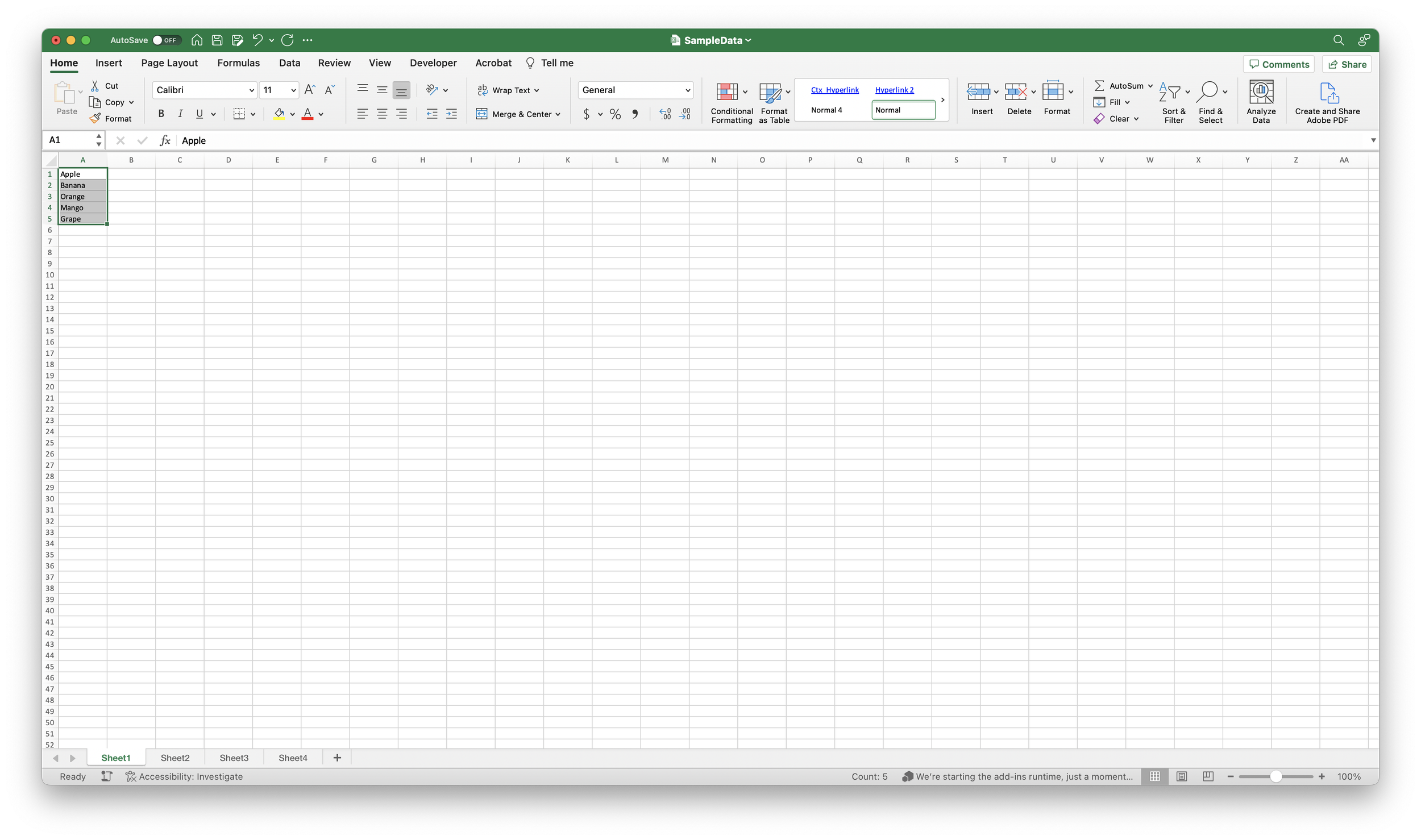
Suppose we have a list of fruits in column A, and we want to find the position of "Orange" in the list.

1. Select an empty cell where you want the result to appear.

2. Enter the following formula in the selected cell:

=MATCH("Orange", A1:A10, 0)

In this example:

• "Orange" is the lookup_value, which is the fruit we want to find.
• A1:A10 is the lookup_array, the range where we want to search for "Orange."

• 0 is the match_type, indicating that we want an exact match.

• Press the "Enter" key to apply the formula.

The MATCH() function will now return the position of "Orange" within the range A1:A10.

Handling Errors:

If the MATCH() function does not find a match for the lookup_value, it returns the #N/A error. To handle this situation and provide a custom message when no match is found, you can use the IFERROR() function. For example:

=IFERROR(MATCH("Orange", A1:A10, 0), "Not Found")

In this modified formula:

• IFERROR() checks if the MATCH() function returns an error.
• If the MATCH() function finds a match, the result is displayed.
• If no match is found, the formula returns "Not Found."

Conclusion:

The MATCH() function in Excel is a valuable tool for performing lookups and locating specific values within a dataset. By using different match_type options, you can control the behavior of the function and tailor it to your specific needs. Whether you are searching for data in sorted or unsorted lists, the MATCH() function provides a flexible and efficient way to perform lookups and retrieve valuable information in Excel.